Count Distinct, Unique And Successive Values Using FREQUENCY()

Happy New Year, folks! And now, without further ado…

In my opinion, one of the hardest worksheet functions to get the hang of is the FREQUENCY() function. For today’s post, I’ve assembled a collection of FREQUENCY() formulae which give a count of distinct, unique or successive values. Please note I’m not claiming any credit for their invention – they’ve been written many times before and were created by people who are much cleverer with formulae than I am!

The syntax of the FREQUENCY() function is given below for reference, but if you would like to learn about it before diving into the examples (which are quite advanced) then I highly recommend Mike Girvin’s Excel Magic Trick 627 video.

1. Syntax

This is taken directly from the MS Excel help file:

FREQUENCY(data_array, bins_array)

• Data_array  Required. An array of or reference to a set of values for which you want to count frequencies. If data_array contains no values, FREQUENCY() returns an array of zeros.
• Bins_array  Required. An array of or reference to intervals into which you want to group the values in data_array. If bins_array contains no values, FREQUENCY() returns the number of elements in data_array.
•  FREQUENCY() is entered as an array formula after you select a range of adjacent cells into which you want the returned distribution to appear.
• The number of elements in the returned array is one more than the number of elements in bins_array. The extra element in the returned array returns the count of any values above the highest interval. For example, when counting three ranges of values (intervals) that are entered into three cells, be sure to enter FREQUENCY() into four cells for the results. The extra cell returns the number of values in data_array that are greater than the third interval value.
• FREQUENCY() ignores blank cells and text.
• Formulas that return arrays must be entered as array formulas.

2. Count Of Distinct Values

The formulae we’re going to explore this section form the backbone of the formulae used throughout the rest of the post, so I’m going to explain them by breaking them into bite-size chunks.

2.1 Numbers only

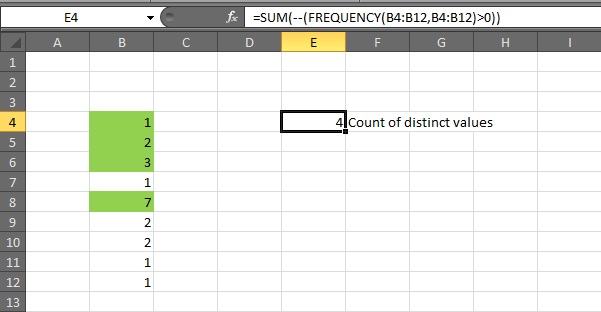
This is one of the simplest formulae we’ll be looking at today. We have a list of numbers in B4:B12 and we want to determine how many distinct values there are.

The distinct numbers in the list are 1, 2, 3 and 7, so the count of distinct numbers is 4. Let’s break the formula down step-by-step to see how it works.

=SUM(--(FREQUENCY(B4:B12,B4:B12)>0))

Firstly, let’s substitute the cell references for the cell values. Note that this formula doesn’t have to be CTRL+SHIFT+ENTER‘d.

=SUM(--(FREQUENCY({1;2;3;1;7;2;2;1;1},{1;2;3;1;7;2;2;1;1})>0))

Next let’s evaluate the FREQUENCY() part of the formula. The key points to this are:

• Duplicated bins return 0.
• There are nine bins but the FREQUENCY() function returns ten values in the array. The last bucket is a count of any values which are greater than the highest specified interval.

=SUM(--({4;3;1;0;1;0;0;0;0;0}>0))

So the four at the start of the array tells us there are four 1s in the list. The three tells us there are three 2s in the list, and so on.

Now, we’re not interested how many 1s, 2s etc there are in the list, just simply that there’s at least one of each of them. We compare every element in the array using >0 to give us an array of logical values.

=SUM(--{TRUE;TRUE;TRUE;FALSE;TRUE;FALSE;FALSE;FALSE;FALSE;FALSE})

Next, the two unary minus operators coerce the TRUE values to 1s and the FALSE values to 0s. We have to do this because SUM() can’t sum logical values in an array or reference but it can sum numbers.

=SUM({1;1;1;0;1;0;0;0;0;0})

Then finally the array is summed to give an answer of 4. 

2.2 Text and/or Numbers

If you want to get a distinct count where text values are to be included then life becomes a little more complicated because FREQUENCY() ignores text values.

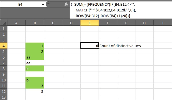
Here’s the array formula from the formula bar:

=SUM(--(FREQUENCY(IF(B4:B12<>"",MATCH("~"&B4:B12,B4:B12&"",0)),ROW(B4:B12)-ROW(B4)+1)>0))

This formula will work fine if your data just contains numbers too, so you might be wondering why I suggested a different formula for the numbers-only scenario in section 2.1: the answer is that this formula is significantly slower (over larger ranges) than the one in 2.1, so use that one when you’ve only got numbers. This theme repeats throughout the post.

Let’s break the formula down:

• Because there is an IF() function inside the FREQUENCY() formula, we have to use a SUM() array formula. To enter an array formula, type it into the formula bar and then press CTRL+SHIFT+ENTER. If done correctly, Excel will automatically surround the formula with { } parentheses. You cannot enter the parentheses manually. You can see the parentheses in the formula bar in the above screenshot.
• The B4:B12<>"" check is used so that blank cells are ignored. It returns this array:{TRUE;TRUE;TRUE;TRUE;TRUE;FALSE;TRUE;TRUE;TRUE}.
• The tilde ~ in the MATCH() function is used as a precaution against a wildcard being the starting character in one of the cells. If you’re sure that your values won’t ever start with these problematic characters (which are * ? and ~) then you can replace "~"& with just ""&. In turn, if you’re certain that your cell values are all text data types then you don’t need the ""& either so you can simply remove the "~"& from the formula altogether. It’s also worth noting that the formula can fail if any of the cells contain a wildcard (particularly *) elsewhere within the text.
• The values in the lookup_array parameter of the MATCH() function are coerced to text data types by using &"". If your cell values are only text data types then you can remove it.

So the MATCH() function returns the position of the first occurrence of each value: {1;2;3;3;5;6;7;8;8}.

Taking the above into account, the IF() part of the formula evaluates to:

IF({TRUE;TRUE;TRUE;TRUE;TRUE;FALSE;TRUE;TRUE;TRUE},{1;2;3;3;5;6;7;8;8})

Which, in turn, evaluates to:

{1;2;3;3;5;FALSE;7;8;8}

The FALSE value corresponds to the blank cell.

Next, the ROW(B4:B12)-ROW(B4)+1 part of the formula returns an array of sequential integers like {1;2;3;4;5;6;7;8;9}, so we can evaluate the formula to:

=SUM(--(FREQUENCY({1;2;3;3;5;FALSE;7;8;8},{1;2;3;4;5;6;7;8;9})>0))

From there, it’s just a case of following the same steps as the previous formula to arrive at a result of 6:

=SUM(--({1;1;2;0;1;0;1;2;0;0}>0))

evaluates to:

=SUM(--{TRUE;TRUE;TRUE;FALSE;TRUE;FALSE;TRUE;TRUE;FALSE;FALSE})

evaluates to:

=SUM({1;1;1;0;1;0;1;1;0;0})

evaluates to:

=6

3. Count Of Unique Values

‘Unique’ values are different to ‘distinct’ values because they are values which only occur once.

3.1 Numbers only

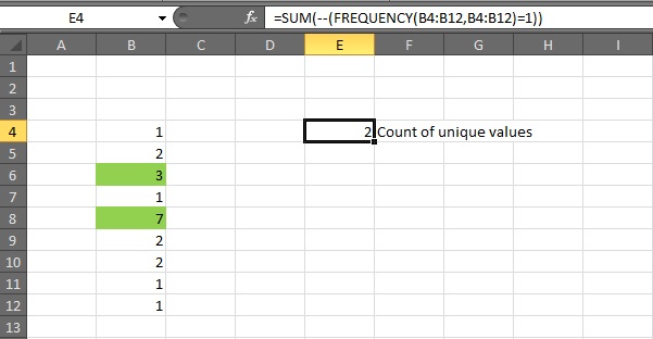
In the below screenshot the unique numbers are 3 and 7.

=SUM(--(FREQUENCY(B4:B12,B4:B12)=1))

This formula is exactly the same as the formula in section 2.1 except that the >0 has been changed to =1. This is because we only want a count of values which occur exactly once.

3.2 Text and/or Numbers

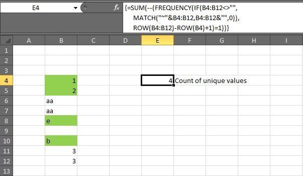
In the screenshot below, the unique values are 1, 2, "e" and "b".

=SUM(--(FREQUENCY(IF(B4:B12<>"",MATCH("~"&B4:B12,B4:B12&"",0)),ROW(B4:B12)-ROW(B4)+1)=1))

This array formula is exactly the same as the array formula in section 2.2 except that the >0 has been changed to =1.

4. Count Of Distinct Values With Condition

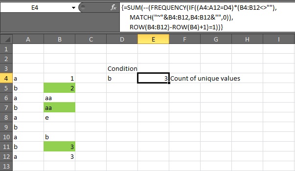
Now we’re going to add an extra condition into our formulae. In the screenshot below, the distinct values corresponding to the letter "b" are 2, "aa" and 3, so we want to calculate a distinct count of 3.

=SUM(--(FREQUENCY(IF((A4:A12=D4)*(B4:B12<>""), MATCH("~"&B4:B12,B4:B12&"",0)),ROW(B4:B12)-ROW(B4)+1)>0))

This formula is very similar to the formula in section 3.2. The only difference is that an extra ‘and’ condition has been specified by including (A4:A12=D4)* in the formula. You can add more ‘and’ conditions if you like by including additional (condition)*.

5. Count Of Unique Values With Condition

Here we have exactly the same values as before, except we want to count only the unique values corresponding to "b". In this case 2, "aa" and 3 only occur once each when they’re on the same row as the letter "b", so we want to calculate a unique count of 3.

=SUM(--(FREQUENCY(IF((A4:A12=D4)*(B4:B12<>""),MATCH("~"&B4:B12,B4:B12&"",0)),ROW(B4:B12)-ROW(B4)+1)=1))

This formula is exactly the same as the formula in section 4 except that the >0 has been changed to =1. This is because we only want a count of values which occur exactly once.

6. Count Of Maximum Occurrences

If we want to get the number of occurrences of a given value from a list then we can use COUNTIF(). But what if we want to get the count of whichever value which occurs the most?

6.1 Numbers only

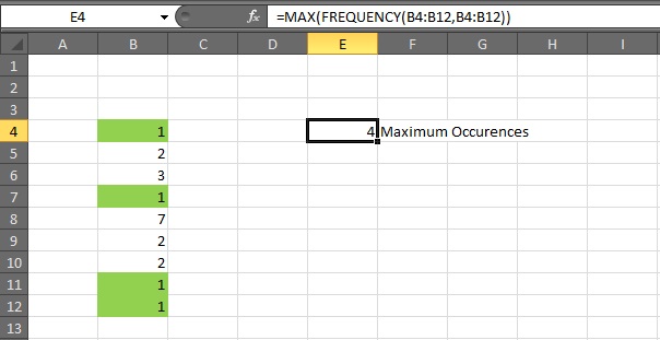
In the screenshot below, the number 1 occurs on four occasions, which is more than any other number.

=MAX(FREQUENCY(B4:B12,B4:B12))

FREQUENCY(B4:B12,B4:B12) returns {4;3;1;0;1;0;0;0;0;0} and the MAX() function takes the largest value from the array.

6.2 Text and/or Numbers

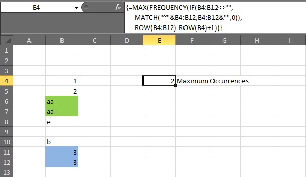
In the screenshot below, the values which occur the most are "aa" and 3, with each occurring twice.

=MAX(FREQUENCY(IF(B4:B12<>"",MATCH("~"&B4:B12,B4:B12&"",0)),ROW(B4:B12)-ROW(B4)+1))

7. Count Of Minimum Occurrences

Getting the minimum number of occurrences isn’t as straightforward as getting the maximum because the FREQUENCY() function returns 0s in the array which we effectively want to ignore because they’re for the duplicate buckets.

7.1 Numbers only

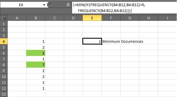
Here the numbers 3 and 7 occur only once, so the minimum number of occurrences should be 1.

=MIN(IF(FREQUENCY(B4:B12,B4:B12)>0,FREQUENCY(B4:B12,B4:B12)))

We work around the problem of the duplicate buckets by checking the values returned by FREQUENCY() and only considering those which are greater than zero. The FREQUENCY() function returns {4;3;1;0;1;0;0;0;0;0} so the formula evaluates to:

=MIN(IF({4;3;1;0;1;0;0;0;0;0}>0,{4;3;1;0;1;0;0;0;0;0}))

Which, in turn, evaluates to:

=MIN({4;3;1;FALSE;1;FALSE;FALSE;FALSE;FALSE;FALSE})

MIN() ignores logical values so it picks up 1 from the array.

7.2 Text and/or Numbers

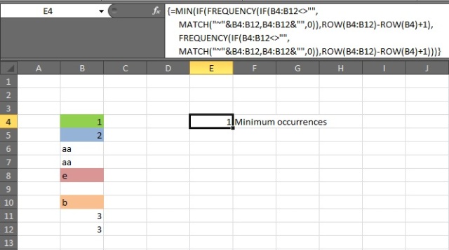
The values 1, 2, "e" and "b" occur only one, so the minimum number of occurrences is 1.

The formula in the formula bar is:

=MIN(IF(FREQUENCY(IF(B4:B12<>"",MATCH("~"&B4:B12,B4:B12&"",0)),ROW(B4:B12)-ROW(B4)+1),FREQUENCY(IF(B4:B12<>"",MATCH("~"&B4:B12,B4:B12&"",0)),ROW(B4:B12)-ROW(B4)+1)))

This evaluates to:

=MIN(IF(FREQUENCY({1;2;3;3;5;FALSE;7;8;8},{1;2;3;4;5;6;7;8;9}),FREQUENCY({1;2;3;3;5;FALSE;7;8;8},{1;2;3;4;5;6;7;8;9})))

then to:

=MIN(IF({1;1;2;0;1;0;1;2;0;0},{1;1;2;0;1;0;1;2;0;0}))

then to:

=MIN({1;1;2;FALSE;1;FALSE;1;2;FALSE;FALSE})

finally arriving at:

=1

8. Maximum Successions Of A Given Value

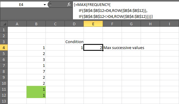
Given the list of numbers below, we want to calculate the largest number of times where the number 1 repeats in succession.

=MAX(FREQUENCY(IF($B$4:$B$12=D4,ROW($B$4:$B$12)),IF($B$4:$B$12<>D4,ROW($B$4:$B$12))))

If we evaluate the IF() functions nested inside the FREQUENCY() function we get:

=MAX(FREQUENCY({4;FALSE;FALSE;7;FALSE;FALSE;FALSE;11;12},{FALSE;5;6;FALSE;8;9;10;FALSE;FALSE}))

This then evaluates to:

=MAX({1;0;1;0;0;2})

The 2 at the end of the array is the largest consecutive count of 1s.

9. Conclusion

As you can see, once you have to start dealing with text values, the FREQUENCY() formulae become much more complicated and slower. When formulae using native functions become long, complicated and slow, they also become prime candidates for conversion into VBA UDFs. With that in mind, next time we’ll have a go at writing a couple of VBA UDFs to count distinct and unique values. In the meantime, do you have any FREQUENCY() formulae you’d like to share?