Conditional Average On Non-Contiguous Ranges Using FREQUENCY()

At the beginning of the year I talked about the FREQUENCY() worksheet function and gave a handful of examples on how it can be used. Today’s article is another, brilliant FREQUENCY() example which was posted by Barry Houdini on the MrExcel board. I’ve picked up quite a few formula tricks from Barry over the years and this one is up there with the best of them. Barry humbly tells me that he in turn picked up the technique from Aladin Akyurek, another expert on the MrExcel board, so full credit to both of them.

The Problem

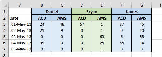
We have some phone call information about three people working in a customer services team.

The count of phone calls is split into two types, ACD and AMS, for each person and we need to get the ACD mean average from the data set. We’ve also been told that the average should not take into account any 0 values in the cells so the correct answer would be 56:

(24 + 21 + 99 + 67 + 87 + 6 + 88) / 7 = 56

In this case we want to do a conditional average: we want to ignore cells which contain 0’s. Usually we could do this by using the AVERAGEIF() function but we can’t do that here because the ACD data is in three separate, or non-contiguous, ranges. This formula will return a #VALUE! error because AVERAGEIF() can’t handle non-contiguous ranges:

=AVERAGEIF((B3:B7,D3:D7,F3:F7),"<>0")

To get an average from a non-contiguous set of ranges we could usually use the SUM() and COUNT() worksheet functions like so:

=SUM(B3:B7,D3:D7,F3:F7)/COUNT(B3:B7,D3:D7,F3:F7)

The problem is the COUNT() will include the 0’s, so the formula returns a result of 26.13 which is incorrect. We could try to adjust the formula to ignore zeros by using COUNTIF() instead of COUNT(), but COUNTIF() can’t be used on non-contiguous ranges either so this will also return #VALUE!:

=SUM(B3:B7,D3:D7,F3:F7)/COUNTIF((B3:B7,D3:D7,F3:F7),"<>0")

So the question is how can we get a count of non-zero values from those cells?

The Solution

The solution Barry posted to this quandary is as follows:

=SUM(B3:B7,D3:D7,F3:F7)/INDEX(FREQUENCY((B3:B7,D3:D7,F3:F7),0),2)

Note that this formula does not need to be CTRL+SHIFT+ENTER’d.

The SUM() part of the formula is straightforward enough, but let’s have a closer look at the rest of it. If you feel that you need a quick refresher on the FREQUENCY() function then take a look at my previous blog entry.

FREQUENCY((B3:B7,D3:D7,F3:F7),0)

The key point is that FREQUENCY() can be used on non-contiguous ranges: the data_array is (B3:B7,D3:D7,F3:F7). The bins_array is 0, so FREQUENCY() will return an array of two values: a count of the ACD numbers which fall into the first bucket of 0, and a count of the ACD numbers which are greater than 0:

FREQUENCY((B3:B7,D3:D7,F3:F7),0)

evaluates to

{8;7}

It’s a safe assumption that there will not be any negative numbers in this particular data set so the 8 is the count of values which are exactly equal to 0 and the 7 is the count of values which are greater than 0. The 7 is the number we’re interested in, so next we use the INDEX() function to extract it from the array:

INDEX({8;7},2)

evaluates to

{7}

and then we divide the sum of the values by 7 to get the correct answer of 56.

SUM(B3:B7,D3:D7,F3:F7)/{7}

evaluates to:

392/{7}

evaluates to our final answer:

{56}

The formula will still work if there are empty cells or even if the non-contiguous ranges are different sizes. Pretty slick.